1. Introduction
We recently implemented the AsyncGRPO algorithm in TRL to decouple inference and training for faster RL training at scale. To validate the implementation, we set up the simplest possible test case:
- Task: Reward =
-len(completion_tokens). The optimal policy emits EOS immediately (reward = -1). - Model: Qwen3-0.6B (28 layers, hidden_dim=1536, vocab=151,936).
def negative_length_reward(completion_ids, **kwargs):
    return [-len(ids) for ids in completion_ids]

trainer = AsyncGRPOTrainer(
    model="Qwen/Qwen3-0.6B",
    args=config,
    train_dataset=dataset,
    reward_funcs=negative_length_reward,
)
trainer.train()
Any working RL algorithm should converge within a handful of steps. Surprisingly, running this script with the default FP32 precision did not converge!
This observation is not isolated. Recent work has flagged numerical precision as a source of instability in RL fine-tuning. Qi et al. (2025) demonstrate that the training-inference mismatch caused by BF16 rounding breaks consistency between the policy that generates rollouts and the policy that computes gradients, and show that reverting to FP16 eliminates the problem. The Megatron-Core MoE report (NVIDIA, 2025) similarly notes that “during reinforcement-learning training, half-precision floating-point (FP16) can deliver greater numerical stability under certain hyper-parameter choices” and provides a dedicated FP16 training path. However, none of these works provide a mechanical explanation of why this mismatch causes training failure. Qi et al. (2025), for example, trace the problem to two intertwined phenomena: the emergence of similar low-rank representations within the attention mechanism and the compounding effect of biased rounding errors inherent in low-precision arithmetic. The paper correctly identifies the phenomena but stops short of providing a full causal chain. Our goal here is to find the why: to dissect, step by step, the exact mechanism through which BF16 precision mismatch corrupts the GRPO gradient and prevents convergence. So what is the root cause? Is it simply a precision mismatch between model weights, or something deeper in the optimizer? As we will show in this (long!) blog post, the answer is a subtle interaction between PPO’s clipping mechanism and the numerical noise introduced by BF16 rounding: the precision gap triggers what we would call a phantom clipping, where the optimizer silences gradient signal for tokens whose policy has not actually changed.
What makes our setting particularly well-suited for studying this problem is its simplicity. The immediate-EOS task has a known optimal policy, a dense scalar reward with no ambiguity, and convergence (or lack thereof) is visible within 100 steps. Combined with the clean, minimal implementation of AsyncGRPO in TRL, this gives us a fully reproducible, easy-to-probe environment where we can isolate and measure precisely where BF16 precision loss enters the training pipeline and how it prevents convergence.
The architecture under study, AsyncGRPO, decouples generation and training: a vLLM inference server generates completions in BF16, asynchronously, while the training process computes gradients and updates weights. When the training forward pass uses a different numerical precision than vLLM, a precision mismatch enters the training pipeline. We will detail exactly how this occurs in the sections that follow.
Before showing the results, let us define the two precision knobs that control the numerical behavior of the training pipeline:
- DTYPE (model weight loading dtype): the precision of the stored model parameters. When set to
float32, the optimizer maintains full-precision weights. When set tobfloat16, the weights themselves are stored in BF16, which means optimizer updates are also accumulated in BF16. - Autocast (torch.amp BF16=True/False): controls whether the forward pass matrix multiplications use hardware-accelerated BF16 GEMMs. When
BF16=True, all matmuls cast their operands to BF16 before execution, matching vLLM’s inference precision.
We ran experiments varying the base weight dtype, the autocast precision, and the learning rate.
Here is a summary table of the experiments:
| DTYPE | Autocast | vLLM | lr | Converges? |
|---|---|---|---|---|
| float32 | BF16=True | BF16 | 1e-6 | Yes |
| float32 | BF16=False | BF16 | 1e-6 | No |
| float32 | BF16=False | FP32 | 1e-6 | Yes |
| float32 | BF16=False | BF16 | 1e-5 | Yes |
| bfloat16 | BF16=True | BF16 | 1e-6 | No |
| bfloat16 | BF16=True | BF16 | 1e-5 | Yes |
| float16 | fp16=True | fp16 | 1e-6 | Yes |
As a sanity check, we repeated the same experiment using the standard synchronous GRPOTrainer (the battle-tested implementation in TRL) instead of our async variant. The results below corroborate the findings: the same convergence behavior appears with the same precision configurations, confirming that the failure is not an artifact of the async architecture but a fundamental property of how FP32/BF16 precision mismatch interacts with the GRPO loss.
The pattern is clear: convergence fails exactly when the training forward pass and the inference engine use different effective precisions, and the learning rate is too small to overcome the resulting mismatch. The rest of this report dissects this failure mechanism in detail.
Before we jump into the core analysis, the next two sections lay the necessary foundations: Section 2 reviews the BF16 floating-point format and where its rounding errors come from, and Section 3 derives the GRPO loss and its gradient so we can later pinpoint exactly where precision loss enters the training pipeline. If you are already familiar with BF16 arithmetic and the GRPO algorithm, feel free to skip ahead to Section 4 — these sections serve as a quick refresher.
- NVIDIA. (2025). Scalable Training of Mixture-of-Experts Models with Megatron Core. arXiv Preprint. https://arxiv.org/abs/2603.07685
- Qi, P., Liu, Z., Zhou, X., Pang, T., Du, C., Lee, W. S., & Lin, M. (2025). Defeating the Training-Inference Mismatch via FP16. arXiv Preprint. https://arxiv.org/abs/2510.26788 back: 1, 2
2. BF16 Arithmetic Introduction
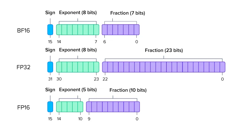
BFloat16 uses 1 sign bit, 8 exponent bits, and 7 fraction (mantissa) bits. Comparison with FP32 and FP16:
2.1 Representable values
A normalized BF16 number has the form:
where is the sign bit, are the 7 fraction bits, and is the 8-bit biased exponent.
The unit in the last place (ULP) at a given magnitude is:
For key magnitudes:
| x | Exponent | ULP | Relative ULP |
|---|---|---|---|
| 1.0 | 0.78% | ||
| 0.5 | 0.78% | ||
| 0.1 | 0.49% | ||
| 0.01 | 0.61% | ||
| 0.001 | 0.76% |
The relative precision is approximately everywhere (7 mantissa bits + 1 implicit leading bit = 8 bits of significand).
2.2 BF16 addition and rounding
Understanding how BF16 addition works is important, because it is the source of silent precision loss during training. When adding two BF16 numbers where , the smaller operand can be partially or entirely lost. The process works as follows:
-
Exponent alignment: ‘s significand is right-shifted to match ‘s exponent. Each shift loses 1 bit. If , all bits of are shifted out and is completely lost.
-
Significand addition: The aligned significands are added.
-
Normalization: Result is shifted to form.
-
Rounding: Result is rounded to 7 fraction bits using “round to nearest, ties to even.”
import torch

W = torch.tensor(1.0, dtype=torch.bfloat16)
dW = torch.tensor(1e-3, dtype=torch.bfloat16)
print(W + dW)
tensor(1., dtype=torch.bfloat16)
If a weight and the update , then . The update is completely annihilated during exponent alignment. The addition returns exactly.
2.3 BF16 boundary crossings
Consecutive BF16 values near are spaced by . A weight “crosses a BF16 boundary” when accumulated FP32 updates push it past the midpoint between two consecutive BF16 values:
At learning rate , with Adam updates per step, the number of steps until the first boundary crossing for a weight of magnitude is approximately:
| Weight mag. | Steps at | Steps at |
|---|---|---|
| 1.0 | 3,906 steps | 391 steps |
| 0.1 | 391 steps | 39 steps |
| 0.01 | 39 steps | 4 steps |
| 0.001 | 4 steps | < 1 step |
At over 100 training steps: only weights with can cross a BF16 boundary. Large-magnitude weights remain frozen in BF16 representation for the entire training run. This means the inference server (vLLM) sees a nearly static model for most parameters, even as the optimizer accumulates meaningful updates in FP32. This mismatch between what training computes and what vLLM serves is the seed of the failure we investigate next.
3. The GRPO Loss and Gradient
To understand where precision loss enters the training pipeline, we need the explicit form of the GRPO gradient. GRPO uses the same clipped surrogate loss as PPO, so we reference PPO’s clipping mechanism throughout this section. The key difference is that GRPO estimates advantages from group-level rewards rather than a learned value network, eliminating the need for a separate critic model.
The clipping mechanism, which is where the precision mismatch does its damage, is identical for both methods.
The key insight from this derivation is that the gradient has three factors, each of which can be corrupted by BF16 rounding in a different way.
3.1 Loss function
The clipped surrogate loss per completion token :
where:
- is the importance sampling ratio, a function of the current policy parameters
- is the advantage (normalized reward per group)
- with
Loss for a sequence of tokens:
3.2 Gradient
The min in the loss selects the more conservative branch, i.e. the one that gives a smaller policy update (more cautious). Differentiating through min yields a gradient only from the active branch (the one currently selected). When the clipped branch is selected, it is constant w.r.t. , so the gradient is zero. Let’s work through a concrete case analysis on the sign of :
- , : selects (constant) → gradient = 0
- , : selects → gradient flows
- , : selects (constant) → gradient = 0
- , : selects → gradient flows
Note the one-sided structure: for only the upper bound clips; for only the lower bound clips. The intuition is that PPO acts as a trust region: “if the policy already moved a lot for this token, stop pushing.” When the ratio exceeds the clip boundary, the gradient is exactly zero for that token. This is correct behavior when the ratio reflects real policy change, but becomes destructive when the ratio is corrupted by precision noise. Define the clipping indicator:
The gradient is then:
Three factors determine the gradient (when ):
- : the advantage. Computed from rewards, independent of precision.
- : the importance weight. Depends on both training-side and vLLM-side log_prob computation, and is differentiated through during backpropagation.
- : the score function (or informant). Depends on the training-side forward and backward precision.
3.3 The score function
The log-probability of token under the model is computed using the language model head (lm_head):
where are the logits, is the final hidden state, and is the vocabulary (151,936 tokens).
The gradient of the log-probability w.r.t. logit :
For the selected token: the gradient is (push logit up). For all other tokens: the gradient is (push logits down).
The gradient w.r.t. a model weight in layer can be computed using the chain rule:
This chain involves backward matmuls through all 28 layers. Each matmul’s precision (BF16) affects the gradient direction by construction.
We now have the three entry points where precision errors can corrupt the gradient: the ratio (through the log-probability difference), the score function (through the backward pass), and the clipping indicator (through the ratio exceeding the trust region). The next section quantifies how large these errors actually are.
- Schulman, J., Wolski, F., Dhariwal, P., Radford, A., & Klimov, O. (2017). Proximal Policy Optimization Algorithms. arXiv Preprint. https://arxiv.org/abs/1707.06347
4. Precision Error Sources
During training, most arithmetic operations in both forward and backward passes are carried out in BF16, although some numerically sensitive operations (e.g., normalization or reductions) are usually computed in higher precision. Because BF16 rounds each value to only 8 significant bits, numerical errors can creep in at every stage of the GRPO pipeline: when computing logits and log-probabilities in the forward pass, when propagating gradients in the backward pass, and when truncating FP32 weights to BF16 at each weight sync with the inference engine. Below we characterize each of these error sources in turn.
4.1 Forward pass logit error
Let’s define:
- = log_probs computed with FP32 matmuls on FP32 weights
- = log_probs computed with BF16 matmuls on weights
Per-matmul error. In a BF16 matmul, each operand is rounded to 8 significant bits, introducing a relative error of at most per value. A single dot product sums products, each with independent error . Since the errors are independent and approximately zero-mean, the variance of the sum is the sum of the variances:
where is the typical magnitude of .
Layer accumulation. Each transformer layer has the residual form . The BF16 rounding error from layer ‘s matmuls enters the residual stream and is carried forward by the skip connection. To first order, the total hidden state error after layers is:
By the CLT argument: approximately independent additive errors grow as .
Combined estimate.
For , : the coefficient is , so the logit error is . The measured value (Section 6) confirms the overall magnitude is .
4.2 Log-probability error
The log-probability of token is a function of the entire logit vector :
Let be the FP32 logits and the per-token logit error from BF16, so .
First-order Taylor expansion:
Differentiating and substituting (see Appendix C for a step-by-step derivation):
The log-prob error is the logit error for the selected token minus the probability-weighted mean logit error across the vocabulary. While log-softmax is shift-invariant (a constant offset added to all logits cancels), BF16 rounding errors are never uniform in practice. The BF16 grid is a step function whose step size (ULP) depends on the exponent of each value. Logits at different magnitudes sit in different exponent bins and get rounded with different step sizes.
4.3 Backward pass gradient error
The backward through layer involves:
In FP32: the matmul is precise. In BF16 autocast: the gradient and weights are rounded to BF16 before multiplication. The per-layer gradient direction error follows the same scaling as the forward pass.
4.4 Weight sync truncation
At each weight sync, training sends FP32 weights to vLLM:
Error per weight: .
Adam’s update rule is . The gradient magnitude cancels, giving regardless of the loss landscape. With , , and , the BF16 representation only changes when accumulated updates cross the midpoint:
In a 100-step training run, this weight never changes in BF16 — exactly the boundary crossing problem described in Section 2.3.
5. The / Decomposition
The previous section catalogued three sites where BF16 rounding errors enter the GRPO pipeline. Regardless of where they originate, all three ultimately manifest in the same place: the log-probabilities the model assigns to each token. Since the GRPO loss depends on the ratio of log-probabilities between the current policy and the rollout policy, every source of BF16 error ultimately feeds into a single difference: .
This motivates decomposing that log-ratio into a component that would exist even under exact BF16 arithmetic and a residual that arises purely from the precision mismatch between training and inference.
Since (the weights vLLM used at rollout time) no longer exists after training progresses to , we decompose by inserting the pivot , a local BF16 forward pass at current weights:
where:
- is the training precision (FP32 or BF16 autocast)
- is the current training weights (FP32)
- is the weights vLLM used to generate the rollout (, where is the tolerated staleness)
This decomposition is measurable: both and can be computed at every training step by running a local BF16 shadow forward pass on the current batch. We detail the implementation of this shadow forward pass in Section 6.1.
5.1 Term : the bf16-aligned ratio
captures everything that changed in BF16 space since the rollout: BF16-visible policy change, vLLM compute path mismatch, etc.
The legitimate importance-sampling correction in async GRPO operates through .
5.2 Term : the precision gap
is the pure local precision gap: how differently the training forward (precision ) and a BF16 forward compute log_probs on the same weights .
If = BF16 (autocast or bf16=True):
Note: is not exactly zero because vLLM’s compute path differs slightly from the training-side transformers implementation (different attention kernels, different fusion patterns), but the residual is negligible in practice.
If = FP32 (no autocast or bf16=False):
From the error analysis in Section 4:
is token-dependent: different tokens activate different weight rows in the LM head, producing different rounding patterns.
The theory predicts for matched precision and for mismatched precision. But is truly random noise that averages out, or does it have structure that systematically corrupts learning? We now have our measuring instrument — a way to separate signal from noise at every training step. Time to examine the evidence.
6. Measuring and in Live Training
6.1 Setup
Two runs on the immediate-EOS task (Qwen3-0.6B, 100 steps, lr=1e-6, BF16 vLLM):
- Run A (converges): DTYPE=float32, BF16=True
- Run B (fails): DTYPE=float32, BF16=False
At each training step, a BF16 shadow forward on the same batch decomposes the log-ratio:
# Compute BF16 shadow log_probs on the same batch (simulates vLLM evaluation)
lp_lowp = self._compute_low_precision_log_probs(model, input_ids, attention_mask, completion_mask)
lp_lowp = lp_lowp[:, : log_probs.shape[1]]

# log_ratio = alpha + beta where:
#   alpha = lp_lowp - old_log_probs  (signal: BF16 policy change since rollout)
#   beta  = log_probs - lp_lowp      (noise: training vs BF16 function mismatch)
alpha = (lp_lowp - old_log_probs)[valid_mask].float()
beta = (log_probs - lp_lowp)[valid_mask].float()

# Log per-step statistics
beta_mean = beta.abs().mean().clamp(min=1e-12)
snr = alpha.abs().mean() / beta_mean
The _compute_low_precision_log_probs helper:
@torch.no_grad()
def _compute_low_precision_log_probs(self, model, input_ids, attention_mask, completion_mask):
    """Run a BF16-autocast forward to simulate what vLLM evaluates."""
    original_forward = getattr(model, "_original_forward", None)
    fwd_fn = original_forward if original_forward is not None else model.forward
    with torch.amp.autocast("cuda", dtype=self._low_precision_dtype):
        outputs = fwd_fn(input_ids=input_ids, attention_mask=attention_mask, use_cache=False)
    logits = outputs.logits[:, :-1, :].float()
    logits.div_(self.temperature)
    return selective_log_softmax(logits, input_ids[:, 1:])
6.2 The precision gap
| Metric | Run B (BF16=False) | Run A (BF16=True) |
|---|---|---|
beta_abs_mean | 0.076 (0.013 to 0.088) | 0.0 exactly (all 100 steps) |
beta_abs_max | 1.83 (0.17 to 3.05) | 0.0 exactly |
beta_mean_signed | -0.0105 (negative bias) | 0.0 |
beta_std | 0.149 (wide spread per token) | 0.0 |
beta_x_adv (correlation with advantage) | +0.0094 (positive correlation) | 0.0 |
For BF16=True, exactly. The autocast training forward and the BF16 shadow produce identical log_probs, confirming the theoretical prediction from Section 5.2.
For BF16=False, is significant and structured:
- Mean magnitude 0.076 with max up to 3.05 for individual tokens.
- Signed mean -0.0105: the FP32 forward systematically produces lower log-probs than BF16, a consistent negative bias, not zero-centered noise.
- Spread std = 0.149: per-token varies widely. Some tokens get (ratio inflated ~16%), others (ratio deflated ~14%).
- Correlation with advantage +0.0094: the precision mismatch systematically over-weights good-advantage tokens and under-weights bad-advantage tokens.
6.3 The bf16-aligned ratio
We now turn to , the component of the log-ratio that reflects actual policy change in BF16 space. If the optimizer is making effective updates, should grow over training as the policy diverges from the rollout policy. The degree to which grows — or fails to grow — tells us how well the training signal is being deployed to the BF16 model that vLLM serves.
| Metric | Run A (BF16=True) | Run B (BF16=False) |
|---|---|---|
| early training | ~0.035 | ~0.035 |
| late training | up to 0.92 | up to 0.33 |
| overall mean | 0.339 | 0.217 |
Both runs start with similar (~0.035). Run A’s grows much larger over time (up to 0.92), indicating the BF16 policy is actively diverging from old rollouts — the model is learning. Run B’s grows more slowly (up to 0.33), suggesting the training signal is less effectively reaching the deployed BF16 weights.
6.4 Signal-to-noise ratio
The individual magnitudes of and are informative, but the quantity that determines whether training can succeed is their ratio. If , the precision noise dominates the true policy change signal — the optimizer is essentially navigating by noise. Conversely, if , the precision gap is a minor perturbation and training can tolerate it.
| Metric | Run A (BF16=True) | Run B (BF16=False) |
|---|---|---|
snr () | 2.82 mean (range 0.42—4.52) |
For BF16=False, . The precision gap is about 1/3 of the total log-ratio magnitude. Early in training (steps 1—3), the SNR is below 1.0, meaning the precision gap dominates.
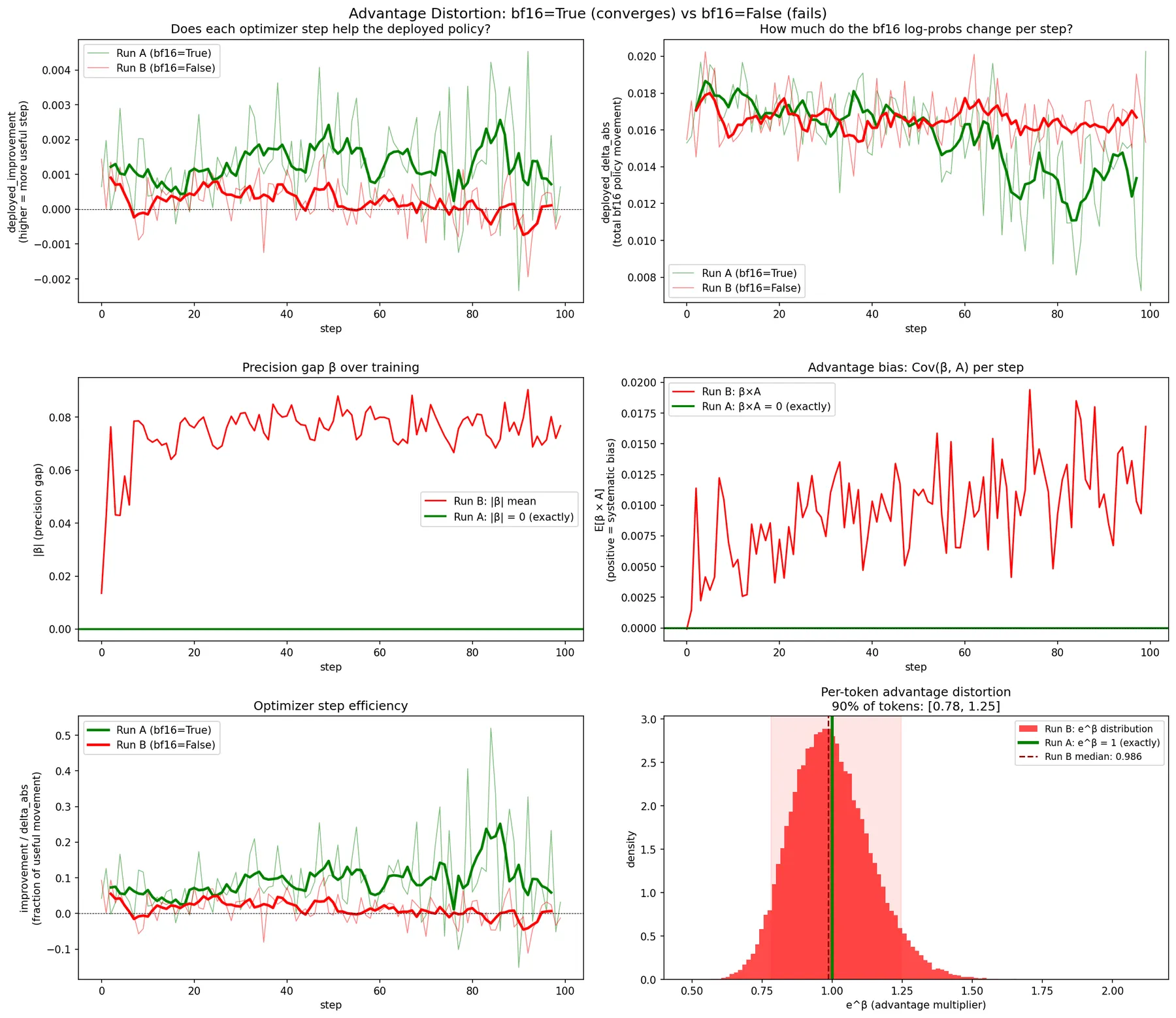
6.5 Deployed improvement per step
The metrics so far describe what the optimizer sees. But the question that matters is: does each optimizer step actually help the deployed BF16 policy?
To measure this directly, we use the same BF16 shadow forward pass introduced in Section 6.1 (the _compute_low_precision_log_probs helper). Before each optimizer step, we record per-token BF16 log-probabilities. After the step, we measure how the BF16 log-probs changed and whether that change is aligned with the advantage direction:
# on_step_end callback — model weights have been updated
lp_after = t._compute_low_precision_log_probs(t.model, input_ids, attention_mask, completion_mask)
delta = (lp_after - lp_before).float()
adv_sign = torch.sign(advantages)
n_valid = valid.sum().clamp(min=1)

# deployed_improvement: did the BF16 log-prob move in the advantage direction?
aligned = (delta * adv_sign * valid.float()).sum() / n_valid
t._metrics["train"]["qat/deployed_improvement"].append(aligned.item())
| Metric | Run A (BF16=True) | Run B (BF16=False) |
|---|---|---|
deployed_improvement mean | +0.00128 | +0.00023 |
deployed_improvement range | -0.0023 to +0.0045 | -0.0020 to +0.0017 |
deployed_delta_abs mean | 0.0156 | 0.0167 |
Each optimizer step improves the BF16 (deployed) policy 5.5x more effectively with BF16=True than with BF16=False. Both settings move the BF16 function by a similar absolute amount per step (~0.016), but the BF16=True movement is much better aligned with the advantage direction. The BF16=False deployed_improvement is barely positive (+0.00023), essentially noise around zero.
6.6 Weight sync boundary crossings
As discussed in Section 2.3, BF16 values are quantized on a grid whose step size (ULP) depends on magnitude. A weight only “moves” in BF16 space when accumulated FP32 updates push it past the midpoint between two consecutive BF16 values. At low learning rates, this can take thousands of steps for large-magnitude weights. We now track the fraction of weights that actually cross a BF16 boundary at each training step, confirming the theoretical estimates from Section 2.3 with empirical measurements.
# Track how many weights actually change their BF16 representation
for n, param in model.named_parameters():
    if param.requires_grad and n in self._last_synced_bf16_weights:
        prev = self._last_synced_bf16_weights[n]
        current_bf16 = param.detach().to(self._low_precision_dtype)
        changed += (current_bf16 != prev).sum().item()
        total += param.numel()

if total > 0:
    self._metrics["train"]["sync/weights_changed_frac"].append(changed / total)
| Metric | Run A (BF16=True) | Run B (BF16=False) |
|---|---|---|
weights_changed_frac mean | 0.29% | 0.24% |
weights_changed_frac first step | 0.96% | 0.96% |
weights_changed_count first step | 7.23M | 7.21M |
weights_changed_count last step | 99K | 55K |
Both runs start with similar boundary crossing rates (~0.96%). Run A maintains a slightly higher crossing rate than Run B at later steps (99K vs 55K), suggesting the BF16=True gradient drives more coherent weight updates.
6.7 Summary of measurements
- is substantial for BF16=False: mean 0.076, ~33% of the total log-ratio.
- is systematically biased: negative mean, positive correlation with advantage.
- Deployed improvement is 5.5x weaker for BF16=False: the optimizer moves weights by the same amount, but the direction is 5.5x less aligned with what helps the deployed policy.
Now that we have an empirical picture of the / decomposition and have measured how the precision gap affects deployed improvement, we need to dive deeper. Models learn through gradients, so to fully understand why the precision mismatch prevents convergence, we need to trace exactly how interacts with the GRPO gradient — and how it distorts the effective training signal.
7. How Corrupts the Gradient
7.1 Closed-form gradient distortion
Define the score function , the direction in weight space that makes token more likely.
The full gradient includes the clipping indicator . In this section we analyze the gradient as if all tokens contribute ( for all ). This isolates the multiplicative and score-function effects of . We revisit this assumption in Section 10.
Under this simplification, the clean gradient (BF16=True, ):
The actual gradient (BF16=False, ):
Substituting and (see Appendix D for the full derivation):
where:
7.2 Effective advantage distortion
The ratio distortion can be absorbed into the advantage:
When (as measured: +0.0094):
| Token type | tendency | Effect on gradient | ||
|---|---|---|---|---|
| Good (short completion) | Over-reinforced | |||
| Bad (long completion) | Under-suppressed |
The gradient loses contrast between good and bad completions. The severity depends on the sign and magnitude of : since is convex, positive values amplify the advantage multiplicatively (e.g., , a 16% boost), while negative values attenuate it (e.g., , a 14% reduction). Because , good-advantage tokens tend to get positive (over-reinforced) while bad-advantage tokens tend to get negative (under-suppressed). The net effect is a systematic compression of the effective advantage spread — the optimizer sees less difference between the best and worst completions than actually exists.
7.3 Measuring the distortion: 4-pass gradient decomposition
To measure and independently, we run four backward passes per training step, each with a different combination of ratio and precision. In all four passes the ratio is detached from the computation graph so we can isolate its effect on the gradient magnitude without it flowing through the backward pass itself.
- Pass A (clean ratio + BF16 backward): Uses the BF16-aligned ratio and runs the backward in BF16 autocast. This yields , the gradient the optimizer would compute if there were no precision mismatch at all.
- Pass B (clean ratio + FP32 backward): Same clean ratio , but runs the backward in FP32. The difference isolates , the error from using FP32 instead of BF16 in the backward pass.
- Pass C (actual ratio + BF16 backward): Uses the full corrupted ratio but runs the backward in BF16. The difference isolates , the error from having in the ratio.
- Pass D (actual ratio + FP32 backward): Both the corrupted ratio and the FP32 backward. This is , the gradient the optimizer actually uses during training.
The decomposition is exact by subtraction: , , and the interaction term can be recovered from .
We run this decomposition on the failing configuration: DTYPE=float32, BF16=False, LR=1e-6.
7.4 Results: relative magnitudes
We first measure the magnitude of each error term relative to the clean gradient. This tells us how large the corruption is (whether introduces a 1% or a 40% perturbation). We also track the cosine similarity between the clean and actual gradients to see whether the overall gradient direction is preserved despite the error.
7.5 Results: direction analysis
Beyond magnitudes, we now examine the geometry of the gradient errors: specifically, how the two error terms relate to the clean gradient direction and to each other. This reveals whether the errors reinforce, cancel, or push the gradient in an entirely different direction.
| Step | |||
|---|---|---|---|
| 0 | -0.098 | +0.100 | -0.372 |
| 10 | -0.105 | -0.149 | -0.586 |
| 30 | +0.219 | -0.465 | -0.671 |
| 50 | -0.169 | -0.148 | -0.602 |
| 90 | +0.011 | -0.472 | -0.533 |
The two errors push in opposite directions (mean cosine -0.579), partially cancelling. Under this simplified decomposition, the overall gradient direction stays at cos > 0.95 with the clean gradient. This suggests the damage may not be in the gradient direction itself, but rather in the per-token weighting.
Remember that these measurements dropped the clipping indicator . When we measure the actual training gradient including PPO clipping (Section 8.4), the cosine similarity drops dramatically to 0.55, pointing to a fundamentally different failure mechanism.
7.6 Advantage distortion trajectory
Having examined the gradient geometry, we now look at the impact on the per-token advantage weighting. How much does distort the effective advantage over the course of training?
The mean advantage distortion grows from 1.4% at step 0 to about 8% at steady state, with worst-case individual tokens reaching 300—500% distortion. The bias is consistently positive and grows over training, confirming the systematic over-reinforcement of good-advantage tokens. However, an 8% mean distortion alone does not explain a complete convergence failure. The gradient direction analysis in Section 7.5 showed cos > 0.95, and the advantage bias, while systematic, is modest in magnitude. Something else must be amplifying this relatively small distortion into a catastrophic failure. We will return to this question in Section 10.
7.7 Deployed improvement
We revisit the deployed improvement metric from Section 6.5, now in the context of the gradient distortion analysis. The question is: given that the gradient direction is largely preserved (cos > 0.95) but the advantage weighting is distorted, does the optimizer still produce useful updates for the deployed BF16 policy?
The results are striking: Run A (BF16=True) achieves a mean deployed improvement of +0.00128 per step, while Run B (BF16=False) manages only +0.00022, a 5.8x reduction. Both runs move the BF16 policy by a similar absolute amount per step (~0.016), but the BF16=False movement is nearly random relative to the advantage direction, yielding only 1.3% optimization efficiency compared to Run A’s 8.2%. The consequence is visible in the reward trajectory: Run A converges from -109 to -20, while Run B stalls between -101 and -96.
7.8 Interim summary
The overall gradient direction stays at cos > 0.95 with the clean gradient because the two errors partially cancel. If the gradient direction is preserved, the failure mechanism must operate through a different channel. Great, case closed? Maybe. This analysis was built on top of a dangerous simplification…
These measurements used custom backward passes under a simplified decomposition (dropping the clipping indicator ). The actual training gradient includes clipping effects. Section 8.4 examines the real training gradient and reveals a dramatically different cosine similarity, which will force us to revisit this conclusion.
8. A Deeper Dive into
The previous section showed that, under a simplified model (no clipping), the overall gradient direction remains surprisingly close to the clean gradient (cos > 0.95). However, several questions remain open: How does evolve as training progresses? Are all tokens equally affected? And critically, does the cos > 0.95 finding hold up when we include the actual PPO clipping mechanism?
We run a diagnostic configuration using the failig run configuration (DTYPE=float32, BF16=False, LR=1e-6) with detailed per-step analysis to answer these questions.
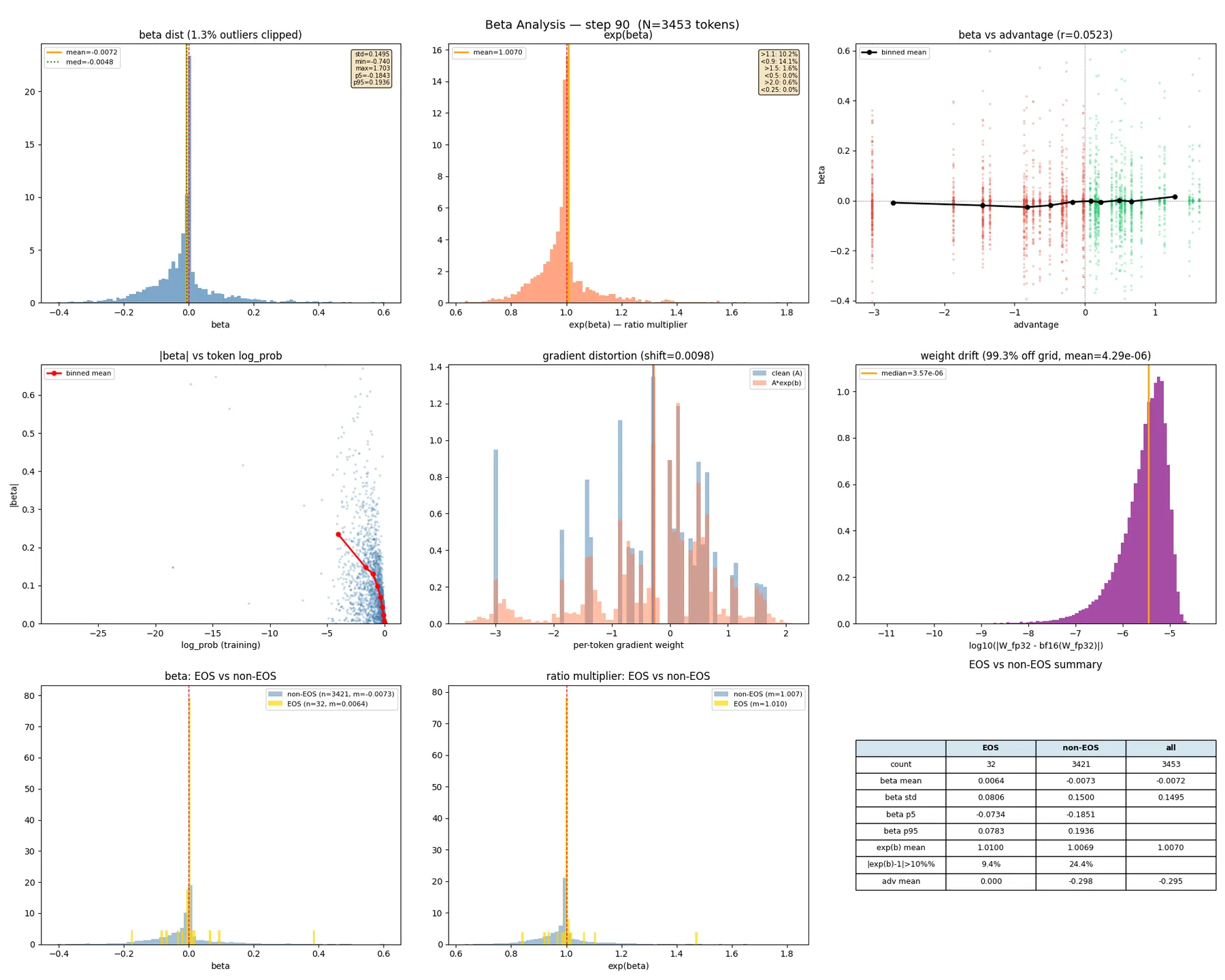
8.1 evolution over training
| Step | mean | std | off by >10% | off by >50% | -adv corr (r) |
|---|---|---|---|---|---|
| 0 | -0.0006 | 0.043 | 1.7% | 0.0% | 0.002 |
| 10 | -0.0156 | 0.091 | 13.3% | 0.3% | 0.015 |
| 30 | -0.0127 | 0.206 | 19.5% | 3.2% | 0.041 |
| 50 | -0.0036 | 0.244 | 25.9% | 4.5% | 0.069 |
Let’s look at the evolution of from step 0 to 50:
- std grows 6x in 50 steps (0.043 to 0.244).
- By step 50, one in four tokens has >10% ratio error, and 1 in 22 has >50% error.
- -advantage correlation grows (0.002 to 0.069): the mismatch becomes increasingly systematic.
Let’s now examine the structure of in relation to token probability. How does the precision gap change with the log-probability that the model assigns to each token?
8.2 Rare tokens have orders-of-magnitude larger
The most revealing finding: tokens with very negative log_probs (rare, low probability) have dramatically larger than common tokens.
At step 50:
- Common tokens (log_prob > -5):
- Moderate tokens (log_prob ~ -10):
- Rare tokens (log_prob < -20): —
This is a 50x difference in mismatch magnitude. The log-probability error is , where the logsumexp is dominated by high-probability tokens, so is relatively stable. For common tokens, errors cancel. For rare tokens, can be very different from , leaving a large residual.
8.3 EOS tokens are mostly spared
EOS is a common token with high probability, and it has a small . The gradient for increasing P(EOS) is relatively clean. But the gradient for suppressing non-EOS tokens is corrupted, especially for rare tokens with the largest values. The model can learn “make EOS more likely” but cannot effectively learn “suppress everything else.”
| Step | EOS mean | EOS std | non-EOS mean | non-EOS std |
|---|---|---|---|---|
| 0 | +0.0018 | 0.007 | -0.0098 | 0.043 |
| 10 | +0.0361 | 0.047 | -0.0218 | 0.122 |
| 50 | +0.0011 | 0.090 | -0.0098 | 0.215 |
8.4 Geometric decomposition: signal vs noise
Section 7.5 found cos > 0.95 using custom backward passes that dropped the clipping indicator. Here we measure the actual training gradient that the optimizer uses, including PPO’s clipping mechanism.
# Save corrupted gradients from the normal training step
corrupted_grads = {name: param.grad.float().clone()
                   for name, param in model.named_parameters() if param.grad is not None}

# Recompute clean REINFORCE loss (no importance sampling ratio)
model.zero_grad()
clean_loss = -(advantages * log_probs * completion_mask).sum() / global_n
clean_loss.backward()

# Compare: cosine similarity and relative L2 error across all parameters
for name, param in model.named_parameters():
    g_corrupt = corrupted_grads[name]
    g_clean = param.grad.float()
    overall_cos_num += (g_corrupt * g_clean).sum()
    overall_cos_den_a += (g_corrupt * g_corrupt).sum()
    overall_cos_den_b += (g_clean * g_clean).sum()
By step 10, the noise component exceeds the signal component (81% vs 58%). This contradicts Section 7.5, which found cos > 0.95. The dramatic drop from cos > 0.95 to cos 0.55 tells us that something about the clipping mechanism interacts with in a way the simplified analysis did not capture.
8.5 Putting the measurements together
| What we measured | Metric | BF16=False | BF16=True | Section |
|---|---|---|---|---|
| Precision gap magnitude | std | 0.15—0.24 | 0 (exact) | 8.1 |
| Fraction of tokens with >10% ratio error | off by >10% | 25% | 0% | 8.1 |
| Rare-token amplification | for log_prob < -20 | 0.5—1.0 | 0 | 8.2 |
| Actual gradient direction | 0.55—0.73 | 1.0 | 8.4 | |
| Gradient noise level | relative L2 error | 0.68—0.85 | 0 | 8.4 |
| Policy improvement per step | deployed improvement | +0.00023 | +0.00128 | 6.5 |
Based on the measurements above, we can formulate an intermediate hypothesis for the failure mechanism. This is not yet a proven causal chain, but it is a theory assembled from the observed experiments that the following sections will test through targeted interventions:
- FP32 weights drift from the BF16 grid: the optimizer accumulates updates in FP32 that are too small to cross BF16 boundaries, creating a growing divergence between the FP32 model and its BF16 representation.
- The log-prob mismatch grows: as FP32 weights drift, the gap between FP32 and BF16 forward passes widens ( std grows 6x in 50 steps).
- Rare tokens are disproportionately affected: tokens with low probability have 50x larger than common tokens, because their logit errors do not cancel with the logsumexp error.
- enters the importance sampling ratio: the corrupted ratio carries precision noise that the optimizer cannot distinguish from real policy change.
- The corrupted ratio distorts the gradient: the effective advantage is compressed, and critically, the actual training gradient (with PPO clipping) shows cos 0.55 with the clean gradient — far worse than the simplified analysis predicted.
- Deployed improvement drops to near zero: each optimizer step moves the BF16 policy by a similar amount, but the movement is nearly random relative to the advantage direction.
- The RL feedback loop amplifies the damage: since the deployed policy barely improves, future rollouts remain low-quality, preventing the signal-to-noise ratio from recovering.
We have assembled a compelling circumstantial case against . But correlation is not causation. To convict , we need a controlled experiment: one that isolates the ratio from the gradient and tests each independently. Is in the ratio truly the cause, or could the FP32 gradient direction alone prevent learning?
9. Confirming Causation: Intervention Experiments
9.1 Setup
To establish whether contamination in the ratio is the primary cause of failure, or whether the FP32 gradient direction independently prevents learning, we design two interventions on the failing configuration:
- Run A (baseline): BF16=True, no intervention. The reference converging run.
- Run B (fails): BF16=False, no intervention. The reference failing run.
- Run F (
ratio_one): BF16=False, but the importance sampling ratio is forced to 1. This reduces GRPO to pure REINFORCE, removing both and from the ratio entirely. - Run G (
ratio_bf16): BF16=False, but the ratio is computed from BF16 shadow log-probs instead of the FP32 training forward. This removes only from the ratio while preserving the legitimate staleness correction .
Critically, Runs F and G keep the FP32 backward pass for gradient computation; only the ratio is changed. This isolates the ratio effect from the gradient direction effect.
9.2 Convergence results
Both interventions converge. Removing from the ratio restores training, even though the gradient direction remains FP32. Runs F and G achieve 16 to 19x higher deployed improvement than Run B, and 2.9—3.5x higher than Run A.
| Run | Converges? | deployed_improvement mean | vs Run B |
|---|---|---|---|
| A (BF16=True) | Yes | +0.00128 | 5.5x |
| B (BF16=False) | No | +0.00023 | 1x |
| F (ratio_one) | Yes | +0.00443 | 19x |
| G (ratio_BF16) | Yes | +0.00366 | 16x |
The FP32 gradient direction, when freed from ratio contamination, is actually more effective at improving the BF16 policy than the BF16 gradient. This definitively rules out the hypothesis that FP32 backward passes independently prevent learning.
9.3 KL divergence
An important question is whether these interventions come at a cost to training stability. PPO’s clipping mechanism exists to enforce a trust region to prevent the policy from diverging too far from the rollout policy. Run F (ratio=1) bypasses this entirely, reducing to pure REINFORCE with no trust region constraint. Run G (ratio_BF16) preserves the trust region through but with a clean ratio. Tracking the KL divergence between the current and rollout policy tells us how aggressively each run moves away from the behavior policy.
| Run | kl mean | kl max |
|---|---|---|
| A | 0.262 | 0.815 |
| B | 0.145 | 0.251 |
| F | 2.558 | 8.499 |
| G | 0.327 | 1.506 |
Run F learns aggressively with KL reaching 8.5 (no PPO clipping constraint). Run G has moderate KL, similar to Run A. The BF16 shadow ratio provides correct importance sampling AND clipping.
9.4 grows large in converging runs
In Runs F and G, the model converges aggressively: it learns to emit EOS with near-certainty, making every other token extremely rare. Recall from Section 8.2 that rare tokens have 50x larger than common tokens, because their logit rounding error sits in a different exponent bin from the probability-weighted mean , leaving a large residual . As the policy becomes peaked, nearly the entire vocabulary becomes “rare,” and explodes on those tokens, pulling the mean up to 9.0. But in these runs, never enters the loss or gradient. The enormous has no effect on training.
In Run B, stays small (0.082) because the model is stuck, the output distribution remains flat, and most tokens have moderate probability with similar rounding behavior.
The interactive visualization below demonstrates this mechanism on a toy 10-token vocabulary with a realistic BF16 rounding model: each token’s logit error scales with the logit’s magnitude (since BF16’s ULP is proportional to the value being rounded), and accumulates through 28 layers. When the model converges and the top token’s logit grows large, its rounding error dominates the logsumexp. Every other token’s then becomes approximately , which can reach very high values. Drag the slider to see this in action:
It is not the magnitude of that causes failure; it is whether enters the ratio.
9.5 Conclusions
We have now assembled all the evidence: contamination in the ratio is the primary cause.
| Condition | in ratio? | Converges? |
|---|---|---|
| BF16=True (Run A) | No () | Yes |
| BF16=False (Run B) | Yes | No |
| BF16=False + ratio=1 (Run F) | No (ratio bypassed) | Yes |
| BF16=False + ratio_BF16 (Run G) | No ( removed) | Yes |
Every run where contaminates the ratio fails. Every run where is absent from the ratio succeeds. The FP32 gradient direction is not just adequate but slightly superior when the ratio is clean.
We have confirmed the what (removing from the ratio fixes training) but not the how. The simplified gradient analysis in Section 7 predicted cos > 0.95 between clean and corrupted gradients, yet the actual gradient with PPO clipping shows cos of only 0.55. Something about the clipping mechanism interacts with in a way we have not accounted for. The next section focuses on isolating the exact mechanism.
10. The Real Mechanism: Phantom Clipping
10.0 Where we stand and what remains unexplained
Section 9 established that in the ratio is the necessary cause, but not how it breaks training. The working hypothesis was multiplicative advantage distortion: reweights the gradient and the gradient loses contrast. However, when we looked at the actual -gradient impact with PPO clipping included (Section 8.4), the cosine similarity dropped from 0.95 to 0.55 — a dramatic discrepancy with the simplified analysis from Section 7.5. This pointed to an interaction with the clipping mechanism that the simplified analysis missed entirely.
10.1 Loss structure experiments
To isolate the clipping interaction, we test four loss variants while keeping intact:
Standard PPO (baseline, fails): flows through both the ratio magnitude and the min/clamp clipping decision.
clipped = torch.clamp(ratio, 1 - eps, 1 + eps)
per_token_loss = -torch.min(ratio * advantages, clipped * advantages)
Detach + center and Detach only: gradient weights detached from the computation graph, eliminating zero-gradient dead zones from min/clamp. Comparing the two tests whether centering (fixing the bias) or detaching (removing dead zones) is what matters.
W = torch.min(ratio * advantages, clipped * advantages)
mu_W = (W * completion_mask).sum() / n_valid
W_centered = W - mu_W
per_token_loss = -W_centered.detach() * log_probs
No-clip (): standard PPO with so large that no token ever hits the clip boundary. flows live through the ratio and gradient, exactly as in the failing baseline. The only difference is that clamp never saturates.
| Run | Loss structure | Converges? | Reward (last 5) | |
|---|---|---|---|---|
| BF16=True | standard PPO | 0.2 | Yes | -28 to -44 |
| BF16=False | standard PPO | 0.2 | No | -92 to -118 |
| BF16=False | detach + center | 0.2 | Yes | -25 to -38 |
| BF16=False | detach only | 0.2 | Yes | -8 to -11 |
| BF16=False | standard PPO | 10.0 | Yes | -23 to -44 |
All three interventions converge. The result is the most informative: standard PPO with fully intact in the ratio and gradient, yet it converges because clipping is disabled. If it converges, the clipping interaction is the mechanism.
10.2 The disproved hypothesis: weight distribution bias
The loss structure experiments show that clipping is involved, but the previous sections also established that systematically biases the effective advantage (). If the multiplicative distortion hypothesis were correct, this bias should manifest in the per-token gradient weights: should be more positive for BF16=False (because inflates good-advantage tokens and deflates bad-advantage tokens). We instrumented the trainer to log and test this prediction directly.
clipped_ratio = torch.clamp(ratio, 1 - eps_low, 1 + eps_high)
W_diag = torch.min(ratio * advantages, clipped_ratio * advantages)
mu_W = (W_diag * completion_mask).sum() / n_valid
| Metric | BF16=True | BF16=False | adv. centering |
|---|---|---|---|
| -0.258 | -0.238 | -0.242 | |
| frac negative | 0.545 | 0.538 | 0.558 |
| imbalance () | 0.525 | 0.547 | 0.527 |
The multiplicative distortion theory is disproved: identically across all runs. The weight distribution is completely unaffected by . Zero bad tokens are reinforced; zero good tokens are suppressed.
10.3 The correct mechanism: phantom clipping
The key to understanding the failure is PPO’s clipping mechanism. When torch.min selects the clipped branch, torch.clamp produces zero gradient because its output is constant. The clipping decision depends on whether the ratio has exceeded the trust region:
| Condition | ||
|---|---|---|
| Gradient = 0 | Gradient flows | |
| Gradient flows | Gradient flows | |
| Gradient flows | Gradient = 0 |
The logic is sound when the ratio reflects real policy change: “if the policy already moved a lot for this token, stop pushing.” But with , the clipping decision uses the corrupted log-ratio. At early training (the policy has barely changed), so the clipping decision reduces to a simple question: is ?
Consider a concrete example. A token has but . The corrupted ratio is . PPO concludes this token has already improved 28% and shuts down its gradient. In reality, the token has not moved at all. The 28% “improvement” is pure precision noise.
PPO sees phantom policy movement from and zeros out the gradient for tokens that still need to learn.
This is the mechanism we have been looking for. Not gradient direction corruption (see Section 7 for the analysis without clipping), not multiplicative advantage distortion (Section 10.2, identical across runs), but a binary, all-or-nothing silencing of tokens that the optimizer still needs to learn from. The clipping indicator , which the simplified analysis dropped, is where does its real damage.
We can quantify how many tokens are affected. From the BF16=False run, at steady state, giving . The empirical clip ratios confirm this prediction:
| Run | clip_ratio (mean) | clip_ratio (step 3) |
|---|---|---|
| BF16=True | 8.5% | 1.0% |
| BF16=False | 15.5% | 13.5% |
| no-clip | 0.1% | 0.0% |
At step 3 the policy has barely moved (), yet BF16=False already clips 13.5% of tokens versus 1.0% for BF16=True. The extra 12.5% are phantom-clipped: tokens whose gradient is silenced purely by precision noise rather than real policy change.
To make this directly visible, we classify every token by comparing the actual ratio against the clean ratio . A token is phantom-clipped if it falls outside the clip boundary under the actual ratio but inside it under the clean ratio. In the interactive visualization below, you can move the step slider to see how many tokens fall outside the PPO clipping zone at each training step. For each step, toggle the Remove beta button to see where the clipped tokens would have been without the artificial noise. They collapse back into the safe zone.
The visualization shows each token positioned by its importance sampling ratio. With the actual ratio (including ), tokens are scattered well beyond the clip boundaries: at step 5, 17.2% of tokens are phantom-clipped while only 0.4% are legitimately clipped. Clicking “remove beta” recomputes the ratio using only , and virtually all tokens snap back to cluster tightly around , well inside the trust region. By step 30 legitimate clipping emerges as the policy begins to move, but phantom clipping (23.7%) still dominates over legitimate clipping (9.5%).
Coming back to Section 7.1’s gradient decomposition, we can now restore the clipping indicator that was previously dropped. This introduces a third error term that captures the phantom clipping effect:
where captures gradient signal gained or lost when flips the clipping decision. At early training (), approximately 13% of tokens lose their gradient entirely.
Three lines of evidence confirm is the dominant failure mechanism:
- Removing clipping () fixes convergence while keeping and fully intact. The multiplicative distortion from remains in the gradient, yet the model converges.
- The weight distribution is unaffected by , ruling out the multiplicative advantage distortion channel entirely (Section 10.2).
- Detaching eliminates through a different route by removing
min/clampfrom the backward path, and also restores convergence.
10.4 Deployed improvement
We now look at the deployed improvement across our loss structure runs:
| Run | deployed_improvement (mean) | deployed_delta_abs (mean) | Efficiency |
|---|---|---|---|
| BF16=True | +0.00125 | 0.01581 | 7.9% |
| BF16=False | +0.00018 | 0.01649 | 1.1% |
| adv. centering | +0.00154 | 0.01557 | 9.9% |
| detach only | +0.00159 | 0.03625 | 4.4% |
| no-clip | +0.00116 | 0.01489 | 7.8% |
The no-clip run recovers to 7.8% efficiency, matching BF16=True’s 7.9%, despite having up to 1.2.
The multiplicative distortion from is tolerable. The phantom clipping is not.
10.5 Comparing the fixes
All successful fixes share one property: they prevent from creating zero-gradient dead zones.
| Fix | How it prevents phantom clipping | KL (last 5) | Stability |
|---|---|---|---|
| BF16=True | , clipping reflects real policy change only | 0.15—0.53 | Stable |
| No token ever reaches the clip boundary | 0.24—1.17 | Moderate | |
| Detach + center | No min/clamp in gradient path | 3.10—5.78 | Less stable |
| Detach only | Same, without centering | 8.71—15.93 | Unstable |
The correct mechanism is phantom clipping: pushes the importance sampling ratio past PPO’s clip boundary for tokens whose policy has not actually changed, triggering torch.clamp saturation and producing exactly zero gradient for those tokens.
11. Conclusion
- Root cause: BF16 precision mismatch between the training forward pass and the vLLM inference server creates a precision gap that enters the importance-sampling ratio.
- Failure mechanism: pushes the ratio past PPO’s clip boundary for tokens whose policy has not actually changed (phantom clipping), silencing ~18% of gradient signal.
- Fix: match precisions (FP16 everywhere, or BF16 autocast), or remove from the policy ratio.
The root cause
Asynchronous GRPO training fails when the training forward pass (FP32) and the vLLM inference server (BF16) use different numerical precision. The precision gap enters the importance-sampling ratio and triggers phantom PPO clipping: the optimizer zeros out gradient signal for tokens whose policy has not actually changed. On a controlled immediate-EOS task with Qwen3-0.6B, this mechanism completely prevents convergence at learning rate , while matched-precision training converges within 100 steps.
The precision gap is not mere numerical noise. It arises from accumulated rounding differences through 28 transformer layers, producing a mean of 0.076 with tails reaching 3.05. The gap is token-dependent (rare tokens have 50x larger ), systematically correlated with the advantage signal (), and large enough to push roughly 18% of tokens past PPO’s clip boundary (). At early training, when the policy has barely moved (), these phantom-clipped tokens receive exactly zero gradient despite genuinely containing useful learning signal. The resulting 7x reduction in deployed improvement per step, combined with the RL feedback loop, locks the system in a permanent stall.
What we ruled out
An initially plausible hypothesis held that corrupts training through multiplicative advantage distortion (), which would compress the effective advantage spread and destroy gradient contrast. We carefully measured this and ultimately disproved it: the per-token gradient weight distribution is identical across all runs regardless of . The decisive experiment was setting (disabling clipping) while leaving fully intact in the ratio and gradient. This run converges to 7.8% deployed improvement efficiency, matching BF16=True’s 7.9%. The multiplicative distortion is tolerable; the phantom clipping is not.
Why RL specifically?
This failure mode is specific to RL. In pretraining and finetuning, enters the cross-entropy loss additively, producing gradient noise that is approximately zero-mean and preserves direction (see Appendix B for a detailed analysis). In RL, the in the importance-sampling ratio converts this additive error into a multiplicative perturbation that interacts destructively with PPO’s clipping mechanism.
All three must co-occur:
- Cross-system ratio: the importance-sampling ratio couples computations at different precisions (training vs inference).
- Clipped surrogate loss: PPO’s clipping creates zero-gradient dead zones that can trigger.
- Closed-loop data: the training data depends on the deployed model, so degraded updates compound over time.
Recommendations
Ranked from strongest to most expedient:
-
FP16 training with FP16 inference. This is the best option when your hardware and framework support it. FP16 has 10 mantissa bits (vs BF16’s 7), giving significantly better numerical stability while still benefiting from hardware-accelerated matmuls. With both training and inference in FP16, the precision mismatch is zero by construction. Our convergence table in Section 1 confirms this: FP16 with matched vLLM converges cleanly at .
-
BF16=True with FP32 master weights. This is the standard mixed-precision recipe used by most LLM training frameworks, and our default recommendation. The autocast matches the training forward pass to vLLM’s BF16, producing . FP32 master weights ensure the optimizer accumulates updates with full precision. This is the safest and most widely supported option.
-
ratio_BF16 (shadow forward pass). When neither FP16 nor BF16 autocast is available, compute the importance-sampling ratio from a BF16 shadow forward pass instead of the FP32 training forward. This removes from the ratio while preserving the FP32 gradient, which (as our intervention experiments showed) is actually slightly more effective than the BF16 gradient when freed from ratio contamination. The cost is one additional forward pass per training step.
-
Disable clipping (). Setting large enough that no token ever reaches the clip boundary eliminates phantom clipping at zero cost. remains in the ratio and gradient, but the multiplicative distortion alone is tolerable. On our simple task this works well; on harder tasks with reward hacking or distribution shift, the lack of a trust region may introduce instability.
-
Detach gradient weights. Removing
min/clampfrom the backward path eliminates zero-gradient dead zones through a different route. This works but produces high KL divergence (up to 15.9) and is the least stable option in practice.
Appendix A: Hypotheses Tested and Their Outcomes
This investigation followed a hypothesis-driven approach. Several claims were tested and either confirmed, partially confirmed, or disproved.
A.1 Hypothesis summary table
| Hypothesis | Claim | Verdict | Key evidence |
|---|---|---|---|
| H1: drowns IS ratio | Partially confirmed | SNR 3. Mechanism is phantom clipping, not multiplicative distortion. | |
| H2: is systematic | Creates a fixed reweighting pattern | Confirmed | Correlated with advantage (+0.0094), rare tokens have 50x larger . |
| H3: FP32 gradient prevents learning | FP32 backward produces wrong gradient | Ruled out | Runs F/G converge with FP32 backward; 16—19x better deployed improvement than Run B. |
| H4: BF16 quantization blocks optimizer | Adam updates too small to cross boundaries | Confirmed (for DTYPE=bfloat16) | ~0.96% boundary crossing rate. Separate failure mode. |
| Multiplicative distortion | biases positive | Disproved | identical across all runs. |
| Phantom clipping | pushes ratios past clip boundary | Confirmed | fixes convergence; 13.5% clip at step 3 vs 1.0%. |
A.2 The multiplicative distortion (detailed analysis)
Sections 7.1—7.7 correctly identified and measured the gradient distortion terms and . Key observations were accurate: gradient direction was largely preserved (cos > 0.95 with the clean gradient). The conclusion that damage is in “the effective advantage ” was on the right track but wrong about the specific mechanism. It is not that wrong tokens get wrong magnitude weights; it is that tokens get zero weight from phantom clipping. The multiplicative effect exists and is measurable, but the experiment proved it is tolerable.
A.3 The gradient direction hypothesis (H3, detailed)
The initial concern was that FP32 backward passes would produce gradient directions misaligned with BF16-optimal updates. The intervention experiments (Runs F and G) definitively ruled this out: when the ratio is clean, FP32 gradients produce 16—19x better deployed improvement than the BF16=False baseline, and 2.9—3.5x better than even the BF16=True run. The FP32 gradient direction is slightly superior, likely because the finer-grained FP32 gradient provides more precise optimization direction for navigating between BF16 boundaries.
A.4 BF16 boundary sign agreement (not predictive)
We hypothesized that corruption would manifest as wrong-direction BF16 boundary crossings. Cross-run comparison reveals the metric is inversely correlated with success:
| Run | Sign agreement (step 60—90) | Converges? |
|---|---|---|
| (no clip) | ~68—72% (worst) | Yes |
| BF16=True (standard PPO) | ~75—78% | Yes |
| BF16=False (standard PPO) | ~77—82% | No |
| detach_only | ~81—86% (best) | Yes |
The metric fails because the REINFORCE baseline conflates legitimate IS divergence (growing with ), -induced corruption, and loss structure differences. The correct proxy for training health is deployed_improvement.
Appendix B: Why Pretraining and Finetuning Are Not Vulnerable
The precision mismatch between training (FP32) and deployment (BF16) is present in BOTH pretraining and RL. Yet pretraining and finetuning converge fine with mixed precision while RL fails. This appendix shows why: in cross-entropy training, enters the loss additively and produces only benign gradient noise, while in RL, enters the importance sampling ratio and interacts destructively with PPO’s clipping mechanism (as shown in the main text).
B.1 Cross-entropy loss under precision mismatch
The standard language modeling objective used in pretraining and finetuning:
With precision mismatch, each log-probability is shifted by the precision gap :
The key point is that enters the loss additively. Taking the gradient:
where is the score function error from computing the backward pass at different precisions.
B.2 Why the additive error is benign
The gradient error in cross-entropy training is a simple additive noise term . This has several properties that make it harmless:
- No per-token reweighting: every token contributes equally to the gradient (). There is no mechanism for to amplify or suppress individual tokens.
- No clipping interaction: cross-entropy has no
min/clampoperations, so there are no zero-gradient dead zones that could trigger. - Approximately zero-mean: the score function errors arise from BF16 rounding, which is approximately unbiased. Averaging over tokens further reduces the noise.
- Gradient direction preserved: the additive noise preserves the overall gradient direction (cos > 0.95 with the clean gradient, as measured in our experiments).
B.3 Why RL is different
In RL (GRPO/PPO), does not enter the loss additively. Instead, it enters through the importance sampling ratio , where the converts the additive log-space error into a multiplicative perturbation. As shown in detail in Sections 7—10 of the main text, this multiplicative perturbation interacts with PPO’s clipping mechanism to produce phantom clipping: tokens whose gradient is zeroed out by precision noise rather than real policy change.
The critical difference is not that reweights tokens (Section 10.2 disproved the multiplicative advantage distortion hypothesis), but that pushes the ratio past the clip boundary, triggering torch.clamp saturation and producing exactly zero gradient for affected tokens.
B.4 The feedback loop
A second factor distinguishes RL from pretraining:
Pretraining is open-loop: the data distribution is fixed. A noisy gradient step does not make the next batch worse. Over many steps, the additive noise averages out.
RL is closed-loop: if the gradient does not improve the BF16 policy, vLLM generates the same completions, rewards carry the same information, and the same corrupted gradient pattern repeats. This creates a self-reinforcing stall that the additive noise in pretraining never triggers.
B.5 Three conditions for precision vulnerability
RL training with precision mismatch fails because three conditions are simultaneously satisfied:
- The loss contains a cross-system ratio. The importance weight couples two computations that may use different precision, and is differentiated through during backpropagation.
- The ratio feeds into a clipped surrogate loss. The triggers PPO’s zero-gradient dead zones for tokens that have not actually changed (phantom clipping).
- The training data depends on the deployed model. The RL feedback loop means gradient signal loss leads to no policy improvement, no data improvement, and permanent stall.
Appendix C: Derivation of the Log-Probability Error Under Logit Perturbation
Claim. To first order, the log-probability error from a logit perturbation is .
Proof. The log-probability of token under the softmax distribution is:
Let be the exact (FP32) logit vector and the elementwise perturbation from BF16 rounding, so the perturbed logits are . Write (1) as where . The first term depends on only when :
For the second term, let . By the chain rule:
Combining (2) and (3):
For the selected token this gives ; for all other tokens it gives . Summing (4) over the full vocabulary confirms shift-invariance: .
Now expand to first order around :
Substituting (4) into (5):
The first sum in (6) collapses (only survives):
The log-probability error equals the logit error of the selected token minus the probability-weighted mean logit error across the vocabulary. If BF16 rounding introduced a uniform shift for all , then by (7): , consistent with the shift-invariance of (4). In practice, BF16 rounding errors are never uniform: the BF16 grid spacing (ULP) depends on the exponent of each logit value, so different logits incur different rounding errors and the residual is generically nonzero.
Appendix D: Derivation of the Gradient Distortion Decomposition
Claim. Under the simplifying assumption (all tokens contribute), the actual gradient decomposes exactly as .
Proof. The GRPO gradient with takes the form , where is the score function at precision and is the advantage. Using the / decomposition from Section 5, the clean and actual gradients are:
Factor the exponential in (2):
Define the score error , so that:
Substituting (3) and (4) into (2):
Distributing the product in (5):
Term (II) is by definition. For term (I), write :
Substituting (7) into term (I) of (6) and recognizing from (1):
The second term in (8) is . Combining (6) and (8):
where:
The decomposition is exact. captures reweighting each token’s contribution through the factor . captures the backward pass precision error . When the clipping indicator is restored, a third term appears (Section 10.3).